
In 2011, Google’s Dremel paper described a query engine that could scan a trillion rows in seconds. That research helped spark a quiet revolution: databases that treat storage and computing power as two separate, elastic resources. Today, the cloud data warehouse is the backbone of modern analytics, and its architecture explains both its greatest strengths and its most expensive surprises.
This article breaks down how these systems are actually built, layer by layer, and what that means for anyone designing, migrating, or paying for one.
What “Cloud Data Warehouse Architecture” Actually Means
A cloud data warehouse is a managed analytical database that runs on rented infrastructure and stores data in a format optimized for large-scale reads rather than transaction-by-transaction writes. Its architecture describes how data is stored, how queries are executed, and how those two pieces talk to each other.
The classic on-premises warehouse (think early Teradata or Oracle appliances) bundled storage and compute into one box. Need more speed? Buy a bigger box. Need more space? Buy a bigger box. The two scaled together whether you needed it or not.
Cloud architecture broke that link. Vendors like Snowflake popularized a multi-cluster shared-data model in which storage sits in cheap object stores while compute runs in independent, resizable clusters. That single design decision reshaped cost models, performance tuning, and even team organization.
For a broader picture of how cloud infrastructure choices play out across providers, see this comparison of AWS vs Azure vs Google Cloud in 2026.
The Three Layers of a Modern Warehouse
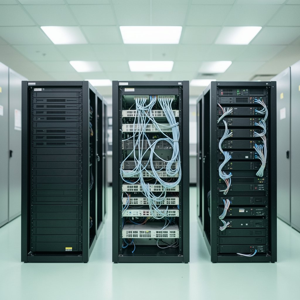
Almost every leading system follows the same conceptual blueprint, even when the marketing language differs.
Layer 1: Storage
Raw data lands in columnar files on distributed object storage. Columnar storage keeps values from the same column together on disk, which means a query that touches three columns out of eighty only reads those three. Combined with compression, this is why analytical scans feel almost magical compared to row-based databases.
Storage is also where the data’s physical layout matters. Partitioning, clustering, and micro-partitioning (Snowflake’s term) determine how much data the engine can skip. Poorly clustered tables are the single most common cause of slow, expensive queries, and no amount of compute scaling fixes bad layout.
Layer 2: Compute
Compute is where queries actually run. These are massively parallel processing (MPP) clusters: many nodes working on slices of the same query simultaneously. Snowflake calls them virtual warehouses; Redshift calls them clusters; BigQuery hides them entirely behind a serverless interface. (Amazon Redshift)
The key architectural property is workload isolation. If the finance team’s heavy month-end job shares compute with the marketing dashboard, everyone suffers. Separate compute clusters per workload solve this, which is why “spin up a new warehouse for the data science team” has become a routine operational move.
Layer 3: Services and Metadata
Above the data sits a control plane: query parsing, optimization, access control, transaction management, and metadata catalogs. This layer decides how a query runs and who is allowed to run it. In serverless systems, it also handles automatic scaling decisions that users never see.
If you want to understand why hyperscalers are building dedicated facilities for this kind of workload, this explainer on what an AI data center is covers the physical side of the story.
Separation of Storage and Compute: Why It Mattered
The separation model sounds like a technical footnote. In practice, it changed three things at once.
Elasticity. Storage grows forever; compute grows for an hour. You can load a decade of history and only pay for heavy processing during the minutes a report runs.
Cost transparency. Because compute is metered separately, teams can see exactly which queries cost money. That visibility is a double-edged sword: it enables FinOps discipline, but it also exposes how often an unoptimized dashboard burns through credits overnight.
Independent failure domains. A runaway query can saturate a compute cluster without corrupting stored data. Storage durability and query performance became separate engineering problems.
The trade-off is real, though. Separating the two means data must move between storage and compute over a network. Vendors invest heavily in caching and local SSD tiers to hide that latency, and query performance often depends more on cache behavior than on raw cluster size.
Columnar Storage and MPP: The Engine Room
Two technologies do most of the heavy lifting inside the compute layer.
| Technology | What it does | Practical effect |
|---|---|---|
| Columnar storage | Stores values by column, not row | Reads only needed columns; compresses 5–10x or more |
| MPP execution | Splits queries across many nodes | Parallel scans and joins on huge tables |
| Vectorized execution | Processes batches of values per CPU cycle | Faster per-core throughput |
| Query optimizer | Rewrites and plans execution | Decides join order, pruning, and parallelism |
| Result caching | Reuses prior query results | Instant repeat queries, lower cost |
The optimizer deserves special attention. Modern warehouses use cost-based optimizers that estimate how many rows each step will touch and pick the cheapest plan. When statistics are stale, those estimates go wrong, and the engine may choose a plan that shuffles terabytes across the network. Regularly refreshing table statistics is unglamorous but decisive.
Early warehouses demanded rigid schemas. Modern ones accept JSON, Parquet, and Avro directly, either through native types (Snowflake’s VARIANT, for example) or external tables that read files sitting in object storage.
That flexibility blurred the line between the data lake (cheap, schema-on-read file storage) and the data warehouse (structured, governed, fast). The hybrid is usually called a lakehouse, though vendors define the term inconsistently. The practical definition: one storage layer holding open file formats, with multiple query engines reading it under a shared catalog.
Open table formats drive this shift. Apache Iceberg provides snapshot isolation, schema evolution, and time travel on plain object storage, letting a warehouse, a Spark cluster, and a streaming job all read the same tables safely. The upside is freedom from lock-in. The downside is that open formats require more operational care than a fully managed proprietary table.
Provisioned vs. Serverless: Two Compute Philosophies
Buyers face a genuine architectural fork here.
Provisioned clusters (classic Redshift, Snowflake virtual warehouses) give you a fixed pool of compute that you size and pay for by the hour or second. Predictable workloads love this. Idle time, however, still costs money unless auto-suspend is configured tightly.
Serverless compute (BigQuery, Redshift Serverless) allocates resources per query. There is nothing to size, but costs fluctuate with usage, and extremely heavy jobs can hit concurrency limits or queue behind other tenants.
| Dimension | Provisioned | Serverless |
|---|---|---|
| Sizing effort | Manual, ongoing | None |
| Cost predictability | High | Variable |
| Idle cost | Yes, unless suspended | None |
| Burst handling | Manual scaling | Automatic |
| Best fit | Steady, known workloads | Spiky, exploratory workloads |
Neither wins universally. Teams commonly run both: provisioned clusters for scheduled pipelines, serverless for ad-hoc analysis.
Security, Governance, and Data Residency
Architecture decisions have compliance consequences. Standard features across major platforms include encryption at rest and in transit, fine-grained role-based access control, row-level and column-level security policies, and audit logging.
Data residency is the architectural constraint people underestimate. Where the storage layer physically sits determines which regulations apply. Regional buildouts are contentious: local opposition to new facilities, such as the Google data center backlash in India in 2026, can affect timelines for regional capacity. Architects should confirm residency guarantees in writing rather than assuming a checkbox covers them.
Practical Tips That Actually Work
After watching many migrations, a few patterns reliably separate smooth rollouts from painful ones.
- Model before you migrate. Lift-and-shift schemas designed for row-based OLTP systems produce bloated, slow warehouses. Redesign around access patterns.
- Set resource monitors on day one. A single unbounded warehouse can generate a shocking bill in a weekend. Budget alerts and hard limits are not optional.
- Right-size clustering keys using real queries. Look at actual WHERE clauses and join keys, not guesses.
- Separate workloads by cluster. Loading, transformation, and BI serving should not compete for the same compute.
- Test with production-scale data. A query that runs in two seconds on a sample can time out on the full table.
- Document cost per dashboard. When teams see the price of their queries, optimization happens without mandates.
The most common mistake is treating the warehouse as a drop-in replacement for an old database. The second most common is over-partitioning: thousands of tiny partitions slow planning and add overhead. Coarse partitions plus good clustering usually beat fine-grained schemes.
If your team is new to analytical workloads, a primer on how to use AI for data analysis can help frame where automated tooling fits and where human modeling judgment still matters.
How the Architecture Affects Everyday Work
Architecture is not abstract. It shows up in daily friction.
When compute and storage are separate, a data engineer can reload a full history table without blocking analysts, because the load runs on its own cluster. When they are coupled, the same job locks the system for hours.
When the catalog is shared, a data scientist can query the same governed tables as the BI team, eliminating the “which version is correct” argument. When catalogs are siloed, duplicate pipelines multiply.
And when cost is metered per query, query design becomes a budget skill. Filtering early, avoiding SELECT *, and materializing expensive intermediate results are no longer style preferences. They are financial controls.
For teams comparing where to keep working data, this breakdown of cloud storage vs local storage differences clarifies which workloads belong where.
Conclusion
Cloud data warehouse architecture comes down to one big idea: storage and compute are separate resources with separate economics. Everything else, from columnar files to MPP clusters to serverless query engines, exists to make that separation fast enough and cheap enough to be practical.
The architecture rewards teams that model data around real access patterns, isolate workloads, and watch costs closely. It punishes teams that lift-and-shift old schemas and assume scale solves design problems. Understand the three layers, respect the optimizer, and treat clustering and cost monitoring as ongoing disciplines rather than one-time setup tasks, and the warehouse will do exactly what it promises: turn enormous datasets into answers in seconds.
Frequently Asked Questions
What is the core principle of cloud data warehouse architecture?
The defining principle is the separation of storage and compute. Data lives in cheap, durable object storage while query processing runs on independent, resizable compute clusters. This lets each resource scale on its own schedule and cost basis, unlike traditional appliances where both grew together.
Is Snowflake or BigQuery better for a cloud data warehouse?
It depends on workload shape. Snowflake offers explicit virtual warehouses that give teams fine control over isolation and sizing, which suits predictable, multi-team environments. BigQuery is fully serverless with no sizing decisions, which suits spiky or exploratory usage. Both separate storage from compute and both support semi-structured data.
What does separation of storage and compute actually change in practice?
Three things: elasticity, cost visibility, and workload isolation. Storage can grow indefinitely while compute spins up only when needed. Because compute is metered separately, teams can attribute spend to specific queries and dashboards. And separate clusters prevent one heavy job from starving everyone else.
What is a lakehouse, and is it the same as a data warehouse?
Not exactly. A lakehouse stores data in open file formats on object storage, governed by a shared catalog, and lets multiple engines query it. A cloud data warehouse is a managed system with its own storage and compute. In practice the two overlap heavily, since most warehouses now read open formats like Apache Iceberg.
Why are my warehouse queries slow even after adding compute?
Scaling compute rarely fixes bad data layout. Common culprits include missing or stale table statistics, poor clustering or partitioning choices, and queries that scan far more columns than needed. Check the query plan and the physical layout before adding clusters.
How do I control costs in a cloud data warehouse?
Set resource monitors and hard limits immediately, separate workloads onto dedicated clusters, enable aggressive auto-suspend, and review the most expensive queries weekly. After that, focus on physical design: better clustering and refreshed statistics reduce scanned bytes, which is where most savings actually live.